
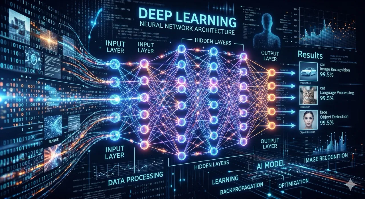
Course Overview
An introductory lecture for anyone who wants to get a real feel for “what deep learning actually is” in one sitting.
It starts with pictures, analogies and interactive demos rather than equations,
and ends by following an MNIST digit classification model step by step, experiencing the whole flow from training to testing to prediction.
flowchart LR
    subgraph Algo["Algorithm (written by humans)"]
        I1["Input\n2"] --> A1["if/else"] --> O1["Output\nGreen"]
    end
    subgraph ML["Machine Learning (learned by the machine)"]
        I2["Input\nImage"] --> A2["w\nweights"] --> O2["Output\nCar"]
    end
    Algo -- "Complexity grows" --> ML
    style I1 fill:#bbdefb,stroke:#1976d2,stroke-width:2px,rx:10,ry:10
    style A1 fill:#eceff1,stroke:#546e7a,stroke-width:2px,rx:10,ry:10
    style O1 fill:#c8e6c9,stroke:#388e3c,stroke-width:2px,rx:10,ry:10
    style I2 fill:#bbdefb,stroke:#1976d2,stroke-width:2px,rx:10,ry:10
    style A2 fill:#fff9c4,stroke:#f9a825,stroke-width:2px,rx:10,ry:10
    style O2 fill:#c8e6c9,stroke:#388e3c,stroke-width:2px,rx:10,ry:10
    style Algo rx:15,ry:15
    style ML rx:15,ry:15
Course Flow
flowchart LR
    subgraph Opening["Opening — Concepts"]
        direction TB
        P1["Part 1\nAlgorithms and Functions"]
        P2["Part 2\nMachine Learning and Deep Learning"]
        P3["Part 3\nNeural Network Structure"]
        P1 --> P2 --> P3
    end
    subgraph Middle["Middle — How Training Works"]
        direction TB
        P4["Part 4\nTraining Analogies\n(Basketball · Blindfolded)"]
        P5["Part 5\nTraining · Validation\n· Test · Prediction"]
        P4 --> P5
    end
    subgraph Closing["Closing — Hands-on Flow"]
        direction TB
        P6["Part 6\nLimits of Deep Learning"]
        P7["Part 7\nHow Models\nAre Chosen"]
        P8["Part 8\nMNIST Walkthrough\n(Dense → CNN)"]
        P6 --> P7 --> P8
    end
    Opening --> Middle --> Closing
    style P1 fill:#e3f2fd,stroke:#90caf9,stroke-width:2px,rx:10,ry:10
    style P2 fill:#e3f2fd,stroke:#90caf9,stroke-width:2px,rx:10,ry:10
    style P3 fill:#e3f2fd,stroke:#90caf9,stroke-width:2px,rx:10,ry:10
    style P4 fill:#fff9c4,stroke:#f9a825,stroke-width:2px,rx:10,ry:10
    style P5 fill:#fff9c4,stroke:#f9a825,stroke-width:2px,rx:10,ry:10
    style P6 fill:#c8e6c9,stroke:#388e3c,stroke-width:2px,rx:10,ry:10
    style P7 fill:#c8e6c9,stroke:#388e3c,stroke-width:2px,rx:10,ry:10
    style P8 fill:#c8e6c9,stroke:#388e3c,stroke-width:2px,rx:10,ry:10
    style Opening rx:15,ry:15
    style Middle rx:15,ry:15
    style Closing rx:15,ry:15
Key Questions
This lecture sets out to answer the following questions.
- What is the difference between an algorithm, machine learning and deep learning?
- Why does classifying a single 28×28 grayscale image involve a nearly infinite number of possibilities?
- What exactly does it mean to “learn the weights
w”? - Why do we need activation functions, and how does softmax turn scores into probabilities?
- How are batch, step and epoch related?
- How do training, validation, test and prediction differ?
- Why do the results change every time you train, even with the same data and the same model?
- What is overfitting, and why can’t deep learning reach 100%?
- What process does a model like “Sonnet 4” go through before it is finally chosen?
Learning Objectives
- Intuitively understand the progression from algorithms → machine learning → deep learning
- Grasp the basic structure of a neural network made of an input layer, hidden layers and an output layer
- Understand the roles of weights, biases and activation functions (ReLU, Softmax)
- Learn the concepts of the loss function, optimizer, learning rate and epoch
- Understand the three-way data split (training/validation/test) and the concept of overfitting
- Understand how a final model is selected by comparing combinations of model architecture, dataset and training
- Experience the full deep learning pipeline (define inputs/outputs → data → model → training → test → prediction) with the MNIST example
Target Audience & Prerequisites
| Target Audience | Prerequisites |
|---|---|
| University students and developers new to deep learning | Programming basics (variables, functions, conditionals) |
| Those who know AI/ML terms but wonder how it all works | A rough idea of matrices and multiplication (optional) |
| Non-majors who want to keep up with where AI is heading | No Python needed (code is explained at the level of its flow) |
Demo Environment
| Item | Setup |
|---|---|
| Framework | TensorFlow / Keras |
| Dataset | MNIST (70,000 handwritten 28×28 digit images) |
| Code execution | Python 3.11+, Jupyter Notebook |
| Model comparison | Single Dense model vs model using Conv2D |
Lecture Structure
Part 1 — Algorithms and Functions
- Function: a processing unit that takes an input and produces an output (input 2 → function → green)
- Algorithm: a person working out how to solve a problem and turning that solution into a computer program
- A simple if/else algorithm example — green if
input < 4, otherwise blue - Key point: humans write the solution themselves — this works well when the input is simple
Part 2 — Machine Learning and Deep Learning
- The nesting of AI ⊃ Machine Learning ⊃ Deep Learning
- Machine learning: instead of a person writing the solution, the machine learns and builds the program
- Why do we need it? Because inputs become complex (images), and the algorithm would have to keep changing with the input
- Number of possibilities for a 28×28 grayscale image: 256^784 ≈ ∞ — an algorithm that handles every case is practically impossible
- Key point: a problem that would need infinitely many variables is solved by approximating it with a finite set of
wweights.- Real natural images occupy only a tiny fraction of that enormous space, so a finite number of weights is enough for a good approximation
Part 3 — Neural Network Structure
- The basic structure of a neural network: input layer → hidden layers → output layer
- Weight: the strength of a connection between nodes. Bias: a value that shifts a node’s output
- Activation function: passes the multiply-and-add result through a nonlinear function, which is what makes stacking layers meaningful
- Hidden layers: ReLU (negatives become 0, positives pass through unchanged)
- Output layer: Softmax (turns multiple outputs into a probability distribution that sums to 1)
- Without activation functions (composing only linear operations), any number of stacked layers is equivalent to a single linear transformation
- Deep Learning = a neural network with many hidden layers stacked deep. Early layers capture simple features (lines, curves); later layers capture abstract features (such as the shape of a digit)
Part 4 — Training Analogies
Two analogies explain how weights are trained.
- Shooting 100 baskets a day: with daily practice, your shots get closer and closer to the hoop.
- “How much harder to throw” is the derivative,
- “How much to change at once” is the learning rate,
- and wind making the same throw land differently is mini-batch noise
- Walking blindfolded: the guide tells the walker which direction to go and how far.
- Measuring the distance is the loss function,
- deciding the direction and stride is the optimizer,
- and the stride length is the learning rate.
- The guide’s directions contain noise, so the walker can’t go in a straight line
- Gradient descent:
- Move the weights little by little against the slope of the loss function until you reach the lowest point.
- If the learning rate is too small, progress is slow; if it is too large, training diverges
Part 5 — Training, Validation, Test and Prediction
- Three-way data split: training (for learning) / validation (monitoring during training) / test (final evaluation).
- If you evaluate on the data you trained on, you can’t tell the model’s real ability
- Softmax: converts the model’s scores (logits) into a probability distribution that sums to 1.
- Small differences in scores are greatly amplified by the exponential function
- Batch: the chunk of data used for a single weight update (typically 32)
- Step: one update that processes one batch.
- 60,000 samples with batch=32 → 1,875 steps per epoch
- Epoch: one full pass over the entire dataset.
- With each additional epoch, the weights become more refined
- Test: measures the model’s generalization performance on data it never saw during training
- Prediction (inference): uses the trained model to infer answers for new data
Part 6 — Does Deep Learning Solve Everything?
- Overfitting: the model fits the training data so closely that it performs worse on data it hasn’t seen before.
- If accuracy drops after adding more epochs, that’s a sign of overfitting
- Bias from training data: the distribution of the training data is the distribution of results the model can produce.
- The case of the PULSE model reconstructing a photo of Obama as a white man
- Differences from model architecture: the same problem can give very different results depending on the model architecture (Bicubic vs SRCNN example)
- Differences from random initialization: training the same model on the same data gives different results every time — because the initial weights are random
- Why it never reaches 100%: noise in the data itself, differences between the training and test distributions, and the trade-off between overfitting and generalization
Part 7 — How Models Are Chosen
- Behind a model released under a single name, such as “Sonnet 4”, lie countless combination experiments
- Architecture variants: internally, several versions with different architectures are built, such as
mark_1,mark_2andmark_3 - Dataset variants: datasets with different collection scopes and cleaning methods are prepared
- Repeated training: even the same combination gives different results each time because of random initialization, so it is trained several times
- Test and selection: average scores are compared on a separate test dataset, and the best combination is released as the final model
- In practice, hyperparameters (learning rate, batch size, number of epochs and so on) are combined as well, so the number of possibilities is far larger
Part 8 — MNIST Walkthrough
We follow the entire deep learning process, divided into six steps.
flowchart TB
    S1["1. Define inputs/outputs"] --> S2["2. Prepare & process dataset"]
    S2 --> S3["3. Build & compile model"]
    S3 --> S4["4. Training and validation"]
    S4 --> S5["5. Test"]
    S5 --> S6["6. Prediction"]
    style S1 fill:#bbdefb,stroke:#1976d2,stroke-width:2px,rx:10,ry:10
    style S2 fill:#bbdefb,stroke:#1976d2,stroke-width:2px,rx:10,ry:10
    style S3 fill:#fff9c4,stroke:#f9a825,stroke-width:2px,rx:10,ry:10
    style S4 fill:#fff9c4,stroke:#f9a825,stroke-width:2px,rx:10,ry:10
    style S5 fill:#c8e6c9,stroke:#388e3c,stroke-width:2px,rx:10,ry:10
style S6 fill:#c8e6c9,stroke:#388e3c,stroke-width:2px,rx:10,ry:10- Define inputs/outputs: input is a 28×28 image → output is probabilities for 10 classes. The loss is
SparseCategoricalCrossentropy - Data: MNIST with 60,000 images (training) + 10,000 images (test). Match integer labels ↔ Sparse and one-hot labels ↔ Categorical
- Model example 1: Input → Flatten → Dense(10, softmax) — 7,850 weights, ~91% accuracy
- Model example 2: Conv2D → MaxPool2D → Conv2D → MaxPool2D → Flatten → Dense — improved accuracy
- Training: normalize inputs (/255.0) → repeat forward → loss → backward → update. Validate with validation_split
- Test: apply the same preprocessing, then evaluate. Compare several model/epoch combinations
- Prediction:
model.predict()→np.argmax()picks the class with the highest probability as the answer
Lecture Format
- Format: In-person/online (1 hour 30 minutes)
- Minimal math: explained mainly through pictures and analogies, with any necessary calculations worked through step by step
- Interactive demos:
- activation function visualizer, neuron calculator, basketball shot training, walking blindfolded,
gradient descent, Softmax visualizer, epoch visualizer, overfitting curve, training simulator,
model selection simulator, MNIST pixel explorer —
11 interactive demos in all
- activation function visualizer, neuron calculator, basketball shot training, walking blindfolded,
- Code sharing: MNIST example code based on TensorFlow/Keras is provided
- Q&A: questions welcome at any time during the lecture, plus a dedicated 10-minute Q&A at the end
Key Messages Summary
| Part | Key Message |
|---|---|
| Part 1 | With an algorithm, humans write the solution themselves. It works well when the input is simple |
| Part 2 | When inputs get complex, humans can’t write out every case. The machine learns and approximates it with weights w |
| Part 3 | A neural network consists of input, hidden and output layers, and stacking layers deep only makes sense with nonlinear activation functions |
| Part 4 | Training means looking at the results and changing the weights little by little. The loss function measures the distance; the optimizer decides the direction and stride |
| Part 5 | Only by splitting data into training/validation/test can you know a model’s real ability (generalization). An epoch is one full pass over the entire dataset |
| Part 6 | Deep learning is not a cure-all. Results vary greatly with overfitting, data bias, model architecture and initial values |
| Part 7 | Behind a single model name lie countless combination experiments of model architecture x dataset x training. The combination with the highest average score on separate test data is released as the final model |
| Part 8 | Dense alone can reach 90%, but adding Conv makes the model more refined. The trade-off among accuracy, speed and memory is what matters |
Contact
For lecture scheduling and pricing inquiries, please reach out via email.